Example reading data: confidence intervals for predictions

In the previous section, we saw that the third model appears to be the most adequate among all three models we have considered. The prediction for this model can be expressed as follows:

\[ \text { Prediction Score }_i=33.3504+6.1522\left(\text { Age }_i-6\right)+5.8103 \text { Group }_i\left(\text { Age }_i-6\right) \]

which corresponds to the expected (or average) score for a child of a certain age in a certain group. But how certain are we about this expected score? To answer this question, we can compute confidence intervals (typically at the 95% confidence level) for our predicted scores. This can be done very similarly to what we did before using the method get_prediction().summary_frame(). First, we recall how the third model is estimated:

import pandas as pd
import matplotlib.pyplot as plt
import statsmodels.formula.api as smf
import numpy as np
from statsmodels.sandbox.regression.predstd import wls_prediction_std

reading = pd.read_csv("https://raw.githubusercontent.com/ELSTE-Master/Data-Science/main/Data/reading.csv")
reading["age_minus_6"] = reading["age"] - 6
mod3 = smf.ols("score ~ age_minus_6 + group:age_minus_6", data=reading).fit()
print(mod3.summary())
                            OLS Regression Results                            
==============================================================================
Dep. Variable:                  score   R-squared:                       0.910
Model:                            OLS   Adj. R-squared:                  0.907
Method:                 Least Squares   F-statistic:                     289.2
Date:                Wed, 12 Nov 2025   Prob (F-statistic):           1.42e-30
Time:                        11:11:29   Log-Likelihood:                -159.47
No. Observations:                  60   AIC:                             324.9
Df Residuals:                      57   BIC:                             331.2
Df Model:                           2                                         
Covariance Type:            nonrobust                                         
==================================================================================================
                                     coef    std err          t      P>|t|      [0.025      0.975]
--------------------------------------------------------------------------------------------------
Intercept                         33.3504      0.790     42.192      0.000      31.768      34.933
age_minus_6                        6.1522      0.260     23.625      0.000       5.631       6.674
group[T.Treatment]:age_minus_6     5.8103      0.716      8.119      0.000       4.377       7.243
==============================================================================
Omnibus:                        0.192   Durbin-Watson:                   2.013
Prob(Omnibus):                  0.909   Jarque-Bera (JB):                0.008
Skew:                           0.027   Prob(JB):                        0.996
Kurtosis:                       3.020   Cond. No.                         5.84
==============================================================================

Notes:
[1] Standard Errors assume that the covariance matrix of the errors is correctly specified.

Suppose we wish to construct the predictions for children of age 6 to 12 in the control group. In the previous slides we saw that this could be done as follows:

# --- Define ages to predict (0:6 corresponds to ages 6 to 12) ---
age_to_predict = np.arange(0, 7)
data_control = pd.DataFrame({"age_minus_6": age_to_predict, "group": "Control"})
pred_control_ci = mod3.get_prediction(data_control).summary_frame(alpha=0.05)

We can inspect the content of the pred_control_ci DataFrame to see what it contains:

pred_control_ci.head(5)
        mean   mean_se  ...  obs_ci_lower  obs_ci_upper
0  33.350442  0.790438  ...     26.083823     40.617061
1  39.502667  0.614987  ...     32.304404     46.700930
2  45.654893  0.516965  ...     38.487601     52.822184
3  51.807118  0.540298  ...     44.632929     58.981307
4  57.959344  0.672471  ...     50.740497     65.178191

[5 rows x 6 columns]
pred_control_ci.columns
Index(['mean', 'mean_se', 'mean_ci_lower', 'mean_ci_upper', 'obs_ci_lower',
       'obs_ci_upper'],
      dtype='object')

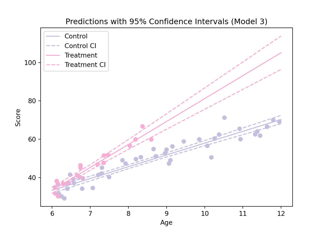
The DataFrame contains the predicted mean scores (mean), the 95% confidence intervals for these means (mean_ci_lower and mean_ci_upper), and also the 95% intervals for individual observations (obs_ci_lower and obs_ci_upper). We can now repeat the same procedure for the treatment group.

data_treatment = pd.DataFrame({"age_minus_6": age_to_predict, "group": "Treatment"})
pred_treatment_ci = mod3.get_prediction(data_treatment).summary_frame(alpha=0.05)

Next, we extract the predicted values and the lower and upper bounds of the confidence intervals, and visualize the predictions alongside the observed data:

# Extract fit, lower, upper
fit_control = pred_control_ci['mean']
lwr_control = pred_control_ci['mean_ci_lower']
upr_control = pred_control_ci['mean_ci_upper']

fit_treatment = pred_treatment_ci['mean']
lwr_treatment = pred_treatment_ci['mean_ci_lower']
upr_treatment = pred_treatment_ci['mean_ci_upper']

# --- Plot predictions with confidence intervals ---
colors = {'Control': '#c4bedf', 'Treatment': '#f6aed5'}
group_col = reading['group'].map(colors)
plt.figure(figsize=(7, 5))
plt.scatter(reading['age'], reading['score'], c=group_col, label=None)

# Control
plt.plot(age_to_predict + 6, fit_control, color=colors['Control'], label="Control")
plt.plot(age_to_predict + 6, lwr_control, color=colors['Control'], linestyle='--', label="Control CI")
plt.plot(age_to_predict + 6, upr_control, color=colors['Control'], linestyle='--')

# Treatment
plt.plot(age_to_predict + 6, fit_treatment, color=colors['Treatment'], label="Treatment")
plt.plot(age_to_predict + 6, lwr_treatment, color=colors['Treatment'], linestyle='--', label="Treatment CI")
plt.plot(age_to_predict + 6, upr_treatment, color=colors['Treatment'], linestyle='--')

plt.xlabel("Age")
plt.ylabel("Score")
plt.title("Predictions with 95% Confidence Intervals (Model 3)")
plt.legend()
plt.show()

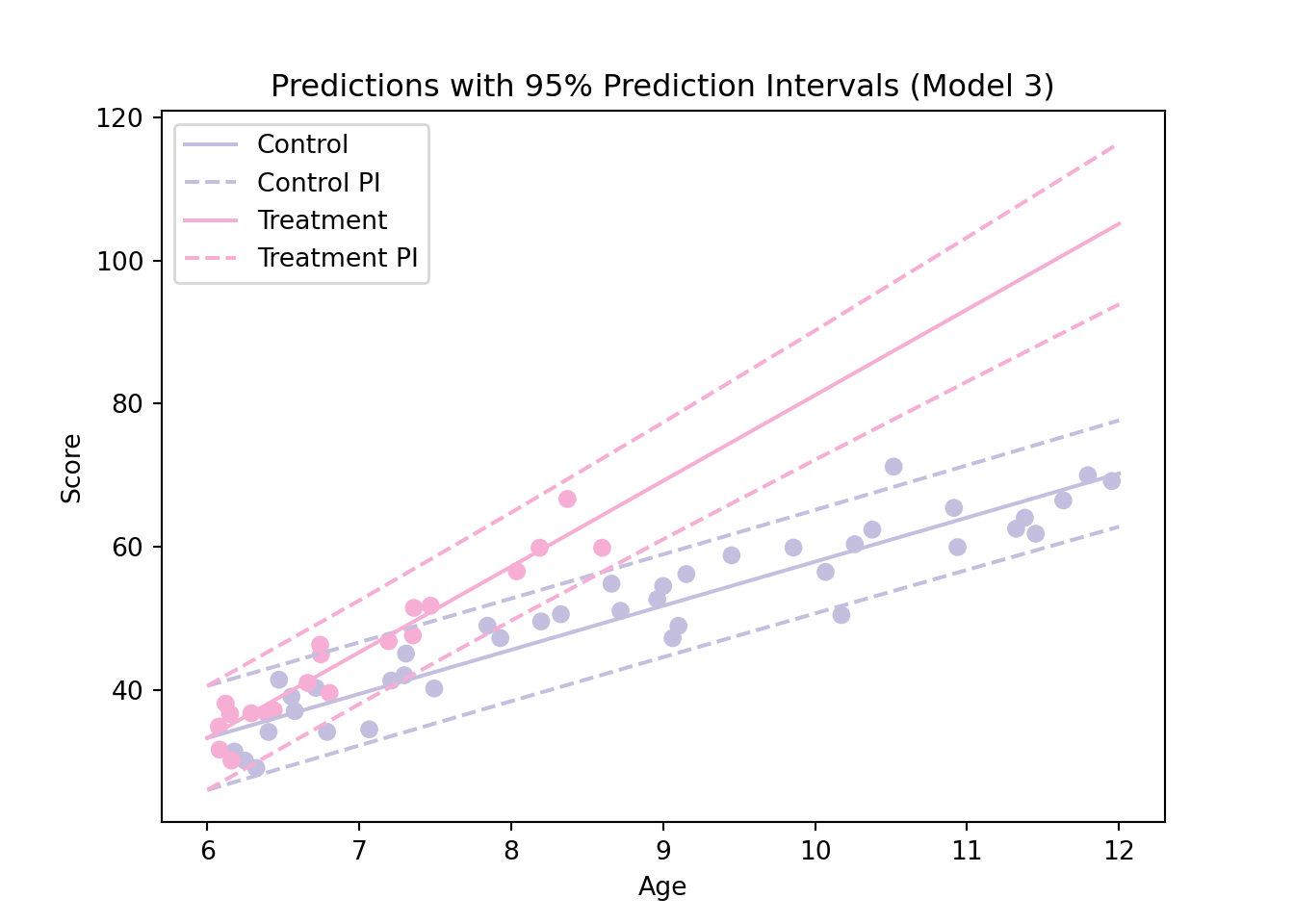
In some situations, it is also of interest to compute a prediction interval, which corresponds to a confidence interval for the score of a child of a certain age and group. This is different from a confidence interval for the mean. Indeed, in the previous graph we can see that many points are outside of the confidence region (which makes sense since the intervals are confidence intervals for the means). These intervals are available directly in the pred_control_ci and pred_treatment_ci objects by using the columns obs_ci_lower and obs_ci_upper.

# Extract confidence intervals for predictions
pred_control_ci[['mean', 'mean_ci_lower', 'mean_ci_upper']].iloc[1]
mean             39.502667
mean_ci_lower    38.271177
mean_ci_upper    40.734158
Name: 1, dtype: float64
# Extract prediction intervals from control group age 7
pred_control_ci[['mean', 'obs_ci_lower', 'obs_ci_upper']].iloc[1]
mean            39.502667
obs_ci_lower    32.304404
obs_ci_upper    46.700930
Name: 1, dtype: float64

In this output, we can see that our prediction intervals are much wider than the previous confidence intervals. For example, for a child of age 7 our predicted score is 39.50267 but the corresponding 95% prediction interval is (32.30440 46.70093). This means that with a probability of 95%, we expect the score of a child of age 7 in the control group to be somewhere between 32.30440 and 46.70093.

Naturally, we can produce a graph similarly to the one we considered previously as follows:

# Extract fit, lower, upper
fit_control = pred_control_ci['mean']
lwr_control = pred_control_ci['obs_ci_lower']
upr_control = pred_control_ci['obs_ci_upper']

fit_treatment = pred_treatment_ci['mean']
lwr_treatment = pred_treatment_ci['obs_ci_lower']
upr_treatment = pred_treatment_ci['obs_ci_upper']

# --- Plot predictions with confidence intervals ---
colors = {'Control': '#c4bedf', 'Treatment': '#f6aed5'}
group_col = reading['group'].map(colors)
plt.figure(figsize=(7, 5))
plt.scatter(reading['age'], reading['score'], c=group_col, label=None)

# Control
plt.plot(age_to_predict + 6, fit_control, color=colors['Control'], label="Control")
plt.plot(age_to_predict + 6, lwr_control, color=colors['Control'], linestyle='--', label="Control PI")
plt.plot(age_to_predict + 6, upr_control, color=colors['Control'], linestyle='--')

# Treatment
plt.plot(age_to_predict + 6, fit_treatment, color=colors['Treatment'], label="Treatment")
plt.plot(age_to_predict + 6, lwr_treatment, color=colors['Treatment'], linestyle='--', label="Treatment PI")
plt.plot(age_to_predict + 6, upr_treatment, color=colors['Treatment'], linestyle='--')

plt.xlabel("Age")
plt.ylabel("Score")
plt.title("Predictions with 95% Prediction Intervals (Model 3)")
plt.legend()
plt.show()