Examples diet data part II

Comparing Diets A, B and C

In this exercise, we will discuss the exercise presented in the last slide of the lecture slides. We will assume that we wish to assess the following claims:

Diet C is the most effective in terms of average weight loss compared to the other two diets.
Diets A and B are comparable in terms of average weight loss.

Therefore, we hope to show that the mean weight loss of diet C is significantly higher than the means of diets A and B. Moreover, the second claim cannot be proven but we hope not to reject the null hypothesis that the means of diets A and B are the same. This would imply that although we can’t prove the means are the same, we don’t have enough evidence to conclude that they are different (which is better than nothing!).

We start by importing the data as presented in the lecture slides.

# Import data
import pandas as pd
diet = pd.read_csv("https://raw.githubusercontent.com/ELSTE-Master/Data-Science/main/Data/diet.csv")

We can now take a look at the data.

# Import data
n = 5
print(diet.head(n)) #print the first n rows of the dataset

   id  gender  age  height diet.type  initial.weight  final.weight
0   1  Female   22     159         A              58          54.2
1   2  Female   46     192         A              60          54.0
2   3  Female   55     170         A              64          63.3
3   4  Female   33     171         A              64          61.1
4   5  Female   50     170         A              65          62.2

To compare the effectiveness of the diets, we first compute the weight loss of the participants (i.e. initial weight - final weight), which can be done in Python as follows:

# Compute weight loss
diet["weight.loss"] = diet["initial.weight"] - diet["final.weight"]

We then construct our “variables of interest”, say dietA, dietB and dietC, by only selecting these diets. This can be done in Python as follows:

# Variable of interest
dietA = diet["weight.loss"][diet["diet.type"]=="A"]
dietB = diet["weight.loss"][diet["diet.type"]=="B"]
dietC = diet["weight.loss"][diet["diet.type"]=="C"]

Next, we construct boxplots to compare the empirical distributions of the three diets as follows:

import matplotlib.pyplot as plt
import numpy as np

plt.figure(figsize=(6,4))

# Boxplot without outliers
plt.boxplot([dietA, dietB, dietC],
            tick_labels=["Diet A", "Diet B", "Diet C"],
            patch_artist=True,
            boxprops=dict(facecolor="lightblue", color="blue"),
            medianprops=dict(color="red"),
            showfliers=False)  # don't show outliers in boxplot

{'whiskers': [<matplotlib.lines.Line2D object at 0x788a589b7a00>, <matplotlib.lines.Line2D object at 0x788a589b7d00>, <matplotlib.lines.Line2D object at 0x788a5876cbb0>, <matplotlib.lines.Line2D object at 0x788a5876cd90>, <matplotlib.lines.Line2D object at 0x788a5876dc00>, <matplotlib.lines.Line2D object at 0x788a5876df00>], 'caps': [<matplotlib.lines.Line2D object at 0x788a589b7fd0>, <matplotlib.lines.Line2D object at 0x788a5876c340>, <matplotlib.lines.Line2D object at 0x788a5876d090>, <matplotlib.lines.Line2D object at 0x788a5876d390>, <matplotlib.lines.Line2D object at 0x788a5876e200>, <matplotlib.lines.Line2D object at 0x788a5876e500>], 'boxes': [<matplotlib.patches.PathPatch object at 0x788a589b66e0>, <matplotlib.patches.PathPatch object at 0x788a5876c5e0>, <matplotlib.patches.PathPatch object at 0x788a5876d630>], 'medians': [<matplotlib.lines.Line2D object at 0x788a5876c640>, <matplotlib.lines.Line2D object at 0x788a5876d690>, <matplotlib.lines.Line2D object at 0x788a58dd79d0>], 'fliers': [], 'means': []}

# Overlay all points with horizontal jitter
for i, data in enumerate([dietA, dietB, dietC], start=1):
    x = np.random.normal(i, 0.09, size=len(data))  # jitter for visibility
    plt.scatter(x, data, alpha=0.7, color='orange', edgecolor='k', zorder=10)

plt.ylabel("Weight loss (kg)")
plt.title("Comparison of Weight Loss for Diets A, B and C")
plt.show()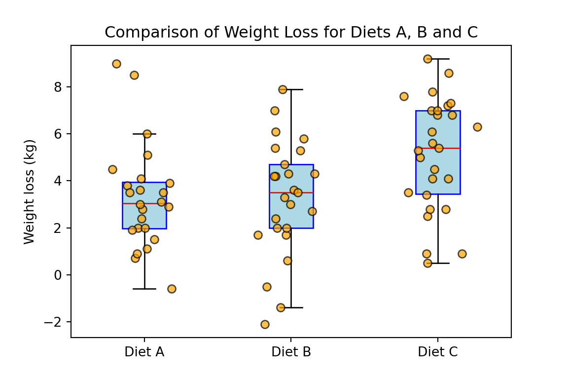

Based on the previous graph, we decide to first employ a Kruskal-Wallis test to assess if the difference of the means of different diets is statistically significant. If we can reject the null hypothesis of this first test, then we will continue with a series of Wilcoxon tests to assess the validity of the two claims discussed at the beginning of this section. However, note that in this example using the Welch’s one-way ANOVA together with the Welch’s t-tests would also be reasonable.

We start with a Kruskal-Wallis test with the following hypotheses:

\[H_{0}: \mu_A=\mu_B=\mu_C \quad \text{and} \quad H_{a}: H_0 \ \text{is false}.\]

where \(\mu_A\), \(\mu_B\) and \(\mu_C\) denote the mean weight loss for diets A, B and C, respectively. As usual, we consider \(\alpha = 0.05\).

The p-value for this first test can be computed as follows:

from scipy.stats import kruskal
H_stat, p_value = kruskal(dietA, dietB, dietC)

print("Kruskal–Wallis H-test results:")

Kruskal–Wallis H-test results:

print(f"H statistic = {H_stat:.3f}")

H statistic = 9.416

print(f"p-value = {p_value:.4f}")

p-value = 0.0090

Thus, at the \(95\%\) confidence level, we can reject the null hypothesis and accept the alternative hypothesis, which allows to conclude that at least one of the means is different from the others. Consequently, we continue our analysis with Wilcoxon tests.

For the second step of our analysis, we consider the following hypotheses which allow us to assess the validity of the claims originally considered:

Test I: \(H_{0}: \mu_A=\mu_B\) and \(H_{a}: \mu_A\neq\mu_B\).

Test II: \(H_{0}: \mu_A=\mu_C\) and \(H_{a}: \mu_A < \mu_C\).

Test III: \(H_{0}: \mu_B=\mu_C\) and \(H_{a}: \mu_B < \mu_C\).

Since we are considering three Wilcoxon tests here, we will compute a corrected \(\alpha\) using Dunn-Sidak correction as follows: \(\alpha_c = 1 - (1 - 0.05)^{1/3} \approx 1.695\%\).

1 - (1 - 0.05)**(1/3)

0.016952427508441503

The p-values for the three previously mentioned tests can be obtained as follows:

from scipy import stats
# Test I: Diet A vs Diet B
stat_AB, p_value_AB = stats.mannwhitneyu(dietA, dietB, alternative ="two-sided")
print("Test I: Diet A vs Diet B")

Test I: Diet A vs Diet B

print("Wilcoxon statistic:", round(stat_AB, 4))

Wilcoxon statistic: 277.0

print("p-value:", round(p_value_AB, 4))

p-value: 0.6526

from scipy import stats
# Test I: Diet A vs Diet C
stat_AC, p_value_AC = stats.mannwhitneyu(dietA, dietC, alternative ="less")
print("Test II: Diet A vs Diet C")

Test II: Diet A vs Diet C

print("Wilcoxon statistic:", round(stat_AC, 4))

Wilcoxon statistic: 180.5

print("p-value:", round(p_value_AC, 4))

p-value: 0.0035

from scipy import stats
# Test I: Diet B vs Diet C
stat_BC, p_value_BC = stats.mannwhitneyu(dietB, dietC, alternative ="less")
print("Test I: Diet B vs Diet C")

Test I: Diet B vs Diet C

print("Wilcoxon statistic:", round(stat_BC, 4))

Wilcoxon statistic: 200.5

print("p-value:", round(p_value_BC, 4))

p-value: 0.0062

Therefore, by rejecting the null hypothesis for both tests II and III, the first claim regarding the larger average weight loss provided by diet C compared to the other two diets is reasonable. Indeed, we can conclude, at the \(95\%\) confidence level, that the mean weight loss of diet C is significant larger than both diets A and B. Moreover, the second claim regarding the similarities of diets A and B in terms of average weight loss is also plausible. While the equivalence can’t be proven, we fail to reject the null hypothesis and therefore it is plausible to say that the two diets have comparable effectiveness in terms of weight loss.