# Import data
import pandas as pd
reading = pd.read_csv("https://raw.githubusercontent.com/ELSTE-Master/Data-Science/main/Data/reading.csv")Example reading data: estimation
In this exercise, we will replicate the analysis of the reading dataset presented in the lectures slides. Our first step is to load the data . We can load the data as follows:
We can now take a look at the data.
# Import data
n = 5
print(reading.head(n)) #print the first n rows of the dataset
id score age group
0 1 59.988809 10.937378 Control
1 2 60.394867 10.261197 Control
2 3 70.023947 11.795009 Control
3 4 41.477072 6.471665 Control
4 5 29.154968 6.321822 ControlComparing groups
To compare the two groups (i.e. Control and Treatment), we can start by comparing the empirical distributions using boxplots similarly to the graph presented in slide 2. For this purpose, we will construct two new variables, called control and treatment, which correspond to the scores in these groups. This can be done as follows:
control = reading['score'][reading['group'] == 'Control']
treatment = reading['score'][reading['group'] == 'Treatment']
Representing the distribution of the score between groups
Using these variables we can easily represent the conditional distribution of the score as follows:
import matplotlib.pyplot as plt

# Create the boxplot
plt.figure(figsize=(6, 5))
plt.boxplot([control, treatment], tick_labels=['Control', 'Treatment']);

# Add labels and title
plt.ylabel('Score')
plt.title('Comparison of Reading Scores by Group')

# Show the plot
plt.show()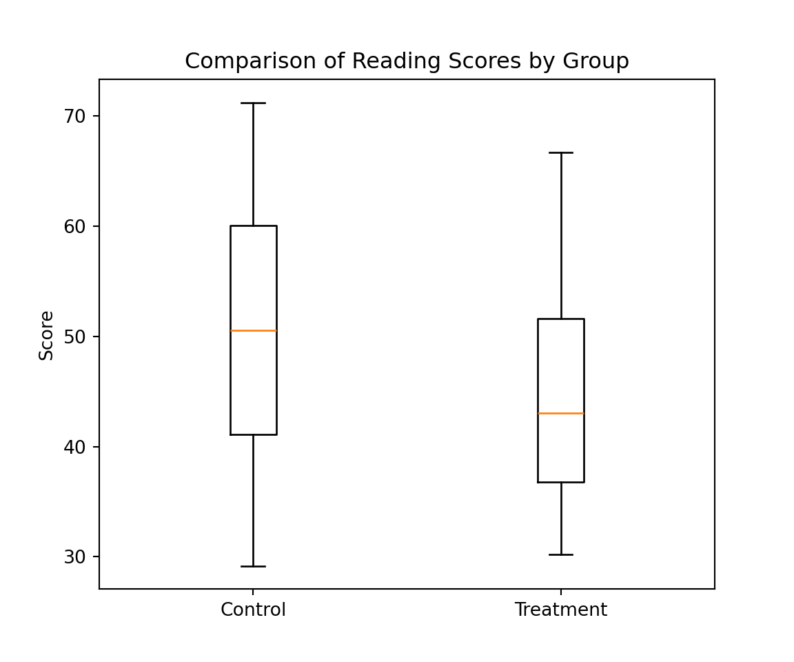
Modelling
As suggested in slide 9, a possible model is given by: \[
\text { Score }_i=\beta_0+\beta_1 \text { Group }_i+\beta_2 \text { Age }_i+\epsilon_i, \quad \epsilon_i \stackrel{i i d}{\sim} \mathcal{N}\left(0, \sigma^2\right)
\] We will refer to this model as “Model 1”. The parameters of this first model can be estimated using the function smf.ols as follows:
import statsmodels.formula.api as smf

# Fit the linear model
mod1 = smf.ols('score ~ group + age', data=reading).fit()
The summary of the fitted model can then be printed with:
# Display the summary
print(mod1.summary())
OLS Regression Results
==============================================================================
Dep. Variable: score R-squared: 0.859
Model: OLS Adj. R-squared: 0.854
Method: Least Squares F-statistic: 173.0
Date: Wed, 12 Nov 2025 Prob (F-statistic): 6.16e-25
Time: 11:11:21 Log-Likelihood: -173.13
No. Observations: 60 AIC: 352.3
Df Residuals: 57 BIC: 358.6
Df Model: 2
Covariance Type: nonrobust
======================================================================================
coef std err t P>|t| [0.025 0.975]
--------------------------------------------------------------------------------------
Intercept -7.8639 3.324 -2.366 0.021 -14.520 -1.208
group[T.Treatment] 6.3771 1.393 4.578 0.000 3.587 9.167
age 6.6457 0.370 17.985 0.000 5.906 7.386
==============================================================================
Omnibus: 0.633 Durbin-Watson: 2.068
Prob(Omnibus): 0.729 Jarque-Bera (JB): 0.386
Skew: 0.196 Prob(JB): 0.824
Kurtosis: 3.013 Cond. No. 50.7
==============================================================================
Notes:
[1] Standard Errors assume that the covariance matrix of the errors is correctly specified.