Intro to Python and Pandas

DataFrames for Data Science

Sébastien Biass

sebastien.biasse@unige.ch

Earth Sciences

Stéphane Guerrier

Stephane.Guerrier@unige.ch

Earth Sciences

Pharmaceutical Sciences

October 15, 2025

Background

We assume that you all followed Guy Simpson’s Python crash course

pandas: A package for data manipulation and analysis handling structured data

Reading/writing data from common formats (CSV, Excel, JSON, etc.)
Handling missing data
Filtering, sorting, reshaping and grouping data
Aggregating data (sum, mean, count, etc.)
Time series support (date ranges, frequency conversions)
Statistical operations

Today’s objectives

Understand what is a pandas DataFrame and its basic anatomy

How to load data in a DataFrame
How to access data → query by label/position
How to filter data → comparison and logical operators
How to rearrange data → sorting values
How to operate on data → arithmetic and string operations

Introduction to pandas

Anatomy of a DataFrame

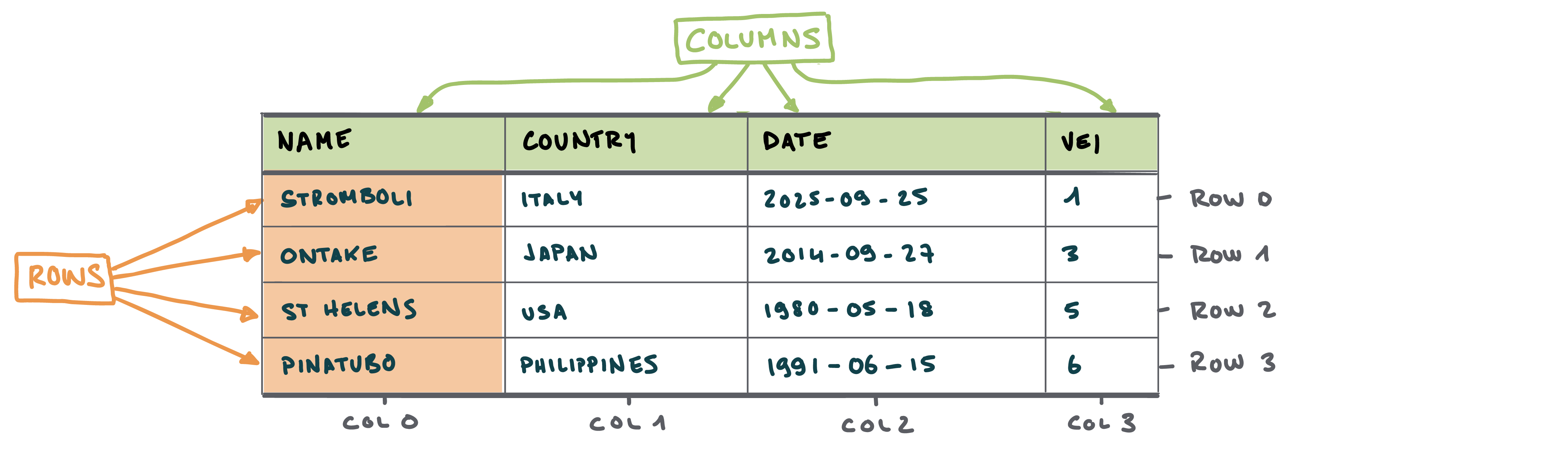
Similar to Excel → contains tabular data composed of rows and columns

In Excel:
- Rows are accessed using numbers
- Columns are accessed using letters

Anatomy of a DataFrame

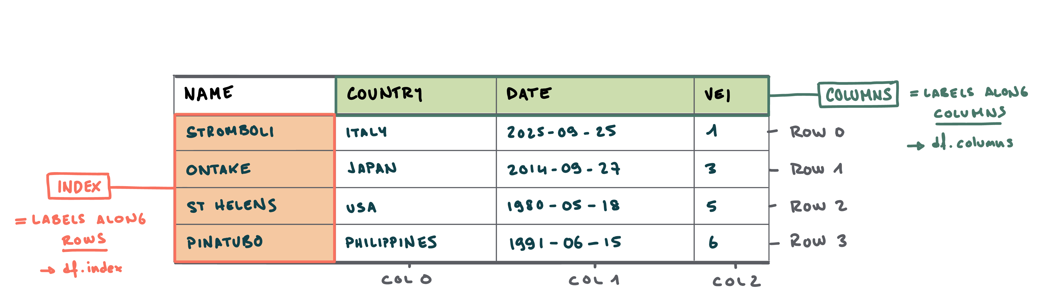
Unlike Excel, rows and columns can be labelled
- Index refers to the label of the rows. In the index, values are usually unique - meaning that each entry has a different label.
- Column refers to the label of - logically - the columns

Data structure

The dataset

Synthetic dataset of selected volcanic eruptions → first 5 rows:

Name	Country	Date	VEI	Latitude	Longitude
St. Helens	USA	1980-05-18	5	46.1914	-122.196
Pinatubo	Philippines	1991-04-02	6	15.1501	120.347
El Chichón	Mexico	1982-03-28	5	17.3559	-93.2233
Galunggung	Indonesia	1982-04-05	4	-7.2567	108.077
Nevado del Ruiz	Colombia	1985-11-13	3	4.895	-75.322

Volcanic explosivity index (VEI)

Setting up the notebook

We start by importing the pandas library
We import it under the name pd - which is faster to type!

# Import the required packages
import pandas as pd

Setting up the notebook

We then load the specified data with the pd.read_csv() function
This returns a DataFrame object in a variable named df

# Import the required packages
import pandas as pd

# Read the data
df = pd.read_csv('https://raw.githubusercontent.com/ELSTE-Master/Data-Science/main/Data/dummy_volcanoes.csv', parse_dates=['Date']) # Load data

Setting up the notebook

We print some data for inspection with df.head()
The functions are now directly called from the DataFrame df object

# Import the required packages
import pandas as pd

# Read the data
df = pd.read_csv('https://raw.githubusercontent.com/ELSTE-Master/Data-Science/main/Data/dummy_volcanoes.csv', parse_dates=['Date']) # Load data

# Show the first 3 rows
df.head(3)

	Name	Country	Date	VEI	Latitude	Longitude
0	St. Helens	USA	1980-05-18	5	46.1914	-122.1956
1	Pinatubo	Philippines	1991-04-02	6	15.1501	120.3465
2	El Chichón	Mexico	1982-03-28	5	17.3559	-93.2233

Setting the index

…for now, the index (→ the first column) is an integer
This might be acceptable in datasets where the label is not important

# Show the first 3 rows
df.head(3)

	Name	Country	Date	VEI	Latitude	Longitude
0	St. Helens	USA	1980-05-18	5	46.1914	-122.1956
1	Pinatubo	Philippines	1991-04-02	6	15.1501	120.3465
2	El Chichón	Mexico	1982-03-28	5	17.3559	-93.2233

Setting the index

Here we want to access the data using the name of the volcano
We set the index using set_index()

# Set the index to the 'Name' column
df = df.set_index('Name')

# Show the first 3 rows
df.head(3)

	Country	Date	VEI	Latitude	Longitude
Name
St. Helens	USA	1980-05-18	5	46.1914	-122.1956
Pinatubo	Philippines	1991-04-02	6	15.1501	120.3465
El Chichón	Mexico	1982-03-28	5	17.3559	-93.2233

Exploring data

Here are some basic functions to review the structure of the dataset:

Function	Description
`df.head()`	Prints the first 5 rows of the DataFrame.
`df.tail()`	Prints the last 5 rows of the DataFrame.
`df.info()`	Displays some info about the DataFrame, including the number of rows (entries) and columns.
`df.shape`	Returns a list containing the number of rows and columns of the DataFrame.
`df.index`	Returns a list containing the index along the rows of the DataFrame.
`df.columns`	Returns a list containing the index along the columns of the DataFrame.

Functions vs attributes

Functions have parentheses → they compute something on df
Attributes do not have parentheses → they store some parameter related to df

Sorting data

Sorting numerical, datetime or strings using .sort_values
Importance of documentation to understand arguments

df.sort_values('VEI').head() # Sort volcanoes by VEI in ascending number

	Country	Date	VEI	Latitude	Longitude
Name
Nyiragongo	DR Congo	2021-05-22	1	-1.5200	29.2500
Ontake	Japan	2014-09-27	2	35.5149	137.4781
Etna	Italy	2021-03-16	2	37.7510	15.0044
Merapi	Indonesia	2023-12-03	2	-7.5407	110.4457
Kīlauea	USA	2018-05-03	2	19.4194	-155.2811

Sorting data

Sorting numerical, datetime or strings using .sort_values
Importance of documentation to understand arguments

df.sort_values('VEI').head() # Sort volcanoes by VEI in ascending number
df.sort_values('Date', ascending=False).head() # Sort volcanoes by eruption dates from recent to old

	Country	Date	VEI	Latitude	Longitude
Name
Merapi	Indonesia	2023-12-03	2	-7.5407	110.4457
Cleveland	USA	2023-05-23	3	52.8250	-169.9444
Sinabung	Indonesia	2023-02-13	3	3.1719	98.3925
Nyiragongo	DR Congo	2021-05-22	1	-1.5200	29.2500
La Soufrière	Saint Vincent	2021-04-09	4	13.2833	-61.3875

Sorting data

Sorting numerical, datetime or strings using .sort_values
Importance of documentation to understand arguments

df.sort_values('VEI').head() # Sort volcanoes by VEI in ascending number
df.sort_values('Date', ascending=False).head() # Sort volcanoes by eruption dates from recent to old
df.sort_values('Country').head() # Also works on strings to sort alphabetically

	Country	Date	VEI	Latitude	Longitude
Name
Calbuco	Chile	2015-04-22	4	-41.2972	-72.6097
Nevado del Ruiz	Colombia	1985-11-13	3	4.8950	-75.3220
Nyiragongo	DR Congo	2021-05-22	1	-1.5200	29.2500
Eyjafjallajökull	Iceland	2010-04-14	4	63.6333	-19.6111
Galunggung	Indonesia	1982-04-05	4	-7.2567	108.0771

Sorting data

Sorting numerical, datetime or strings using .sort_values
Importance of documentation to understand arguments

df.sort_values('VEI').head() # Sort volcanoes by VEI in ascending number
df.sort_values('Date', ascending=False).head() # Sort volcanoes by eruption dates from recent to old
df.sort_values('Country').head() # Also works on strings to sort alphabetically
df.sort_values(['Latitude', 'Longitude']).head() # Sorting using multiple columns

	Country	Date	VEI	Latitude	Longitude
Name
Calbuco	Chile	2015-04-22	4	-41.2972	-72.6097
Agung	Indonesia	2017-11-21	3	-8.3422	115.5083
Merapi	Indonesia	2023-12-03	2	-7.5407	110.4457
Galunggung	Indonesia	1982-04-05	4	-7.2567	108.0771
Tavurvur	Papua New Guinea	2014-08-29	3	-4.3494	152.2847

Your turn!

Go to https://elste-master.github.io/Data-Science/
- Class 1 > Data Structure

Querying data

Accessing data in a DataFrame

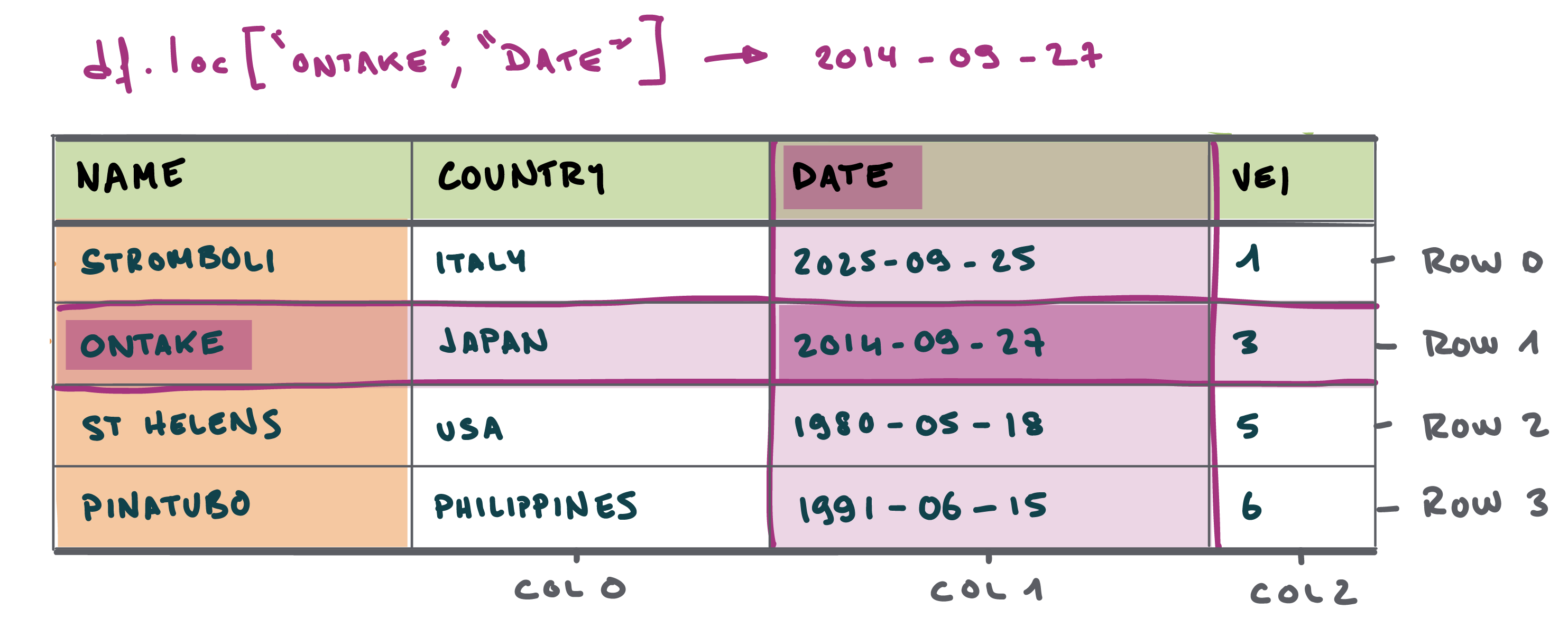
Option 1: label-based indexing

Use the labels of index and columns to retrieve data
Function to use: df.loc

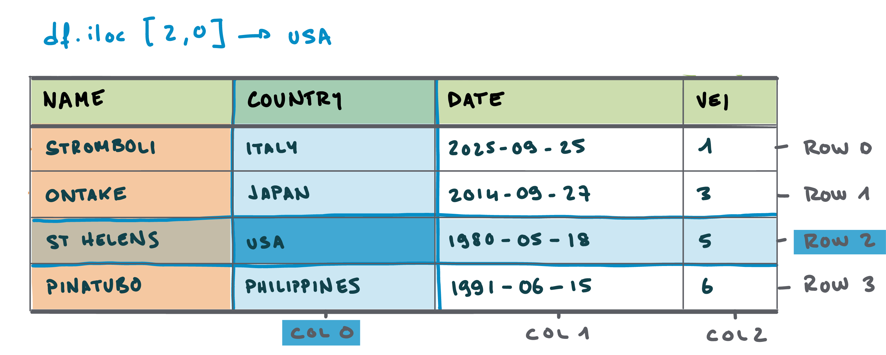
Accessing data in a DataFrame

Option 2: position-based indexing

Use the positions of index and columns to retrieve data
Function to use: df.iloc

Label-based indexing: Rows

Query a row with .loc → Use square brackets [ ]
- Query the row for which the index label is Calbuco
- Returns all columns

df.loc['Calbuco']

Country                    Chile
Date         2015-04-22 00:00:00
VEI                            4
Latitude                -41.2972
Longitude               -72.6097
Name: Calbuco, dtype: object

→ Returns a pd.Series

df.loc[['Calbuco']]

	Country	Date	VEI	Latitude	Longitude
Name
Calbuco	Chile	2015-04-22	4	-41.2972	-72.6097

→ Returns a pd.DataFrame

Label-based indexing: Rows

Query multiple rows with .loc
- Query the rows for which the index labels are Calbuco or Taal
- Returns all columns

df.loc[['Calbuco', 'Taal']]

	Country	Date	VEI	Latitude	Longitude
Name
Calbuco	Chile	2015-04-22	4	-41.2972	-72.6097
Taal	Philippines	2020-01-12	4	14.0020	120.9934

Label-based indexing: Columns

Query columns
- Query the columns for which the column labels are Country or VEI
- Returns all rows

Option 1: with .loc:

df.loc[:, ['Country', 'VEI']].head(3)

	Country	VEI
Name
St. Helens	USA	5
Pinatubo	Philippines	6
El Chichón	Mexico	5

Option 2: without .loc:

df[['Country', 'VEI']].head(3)

	Country	VEI
Name
St. Helens	USA	5
Pinatubo	Philippines	6
El Chichón	Mexico	5

Label-based indexing: Rows and Columns

Again, choice on whether to use .loc to query columns

Option 1: Columns are specified inside .loc:

df.loc[['Calbuco', 'Taal'], ['Country', 'VEI']].head(3)

	Country	VEI
Name
Calbuco	Chile	4
Taal	Philippines	4

Option 2: Columns are specified outside .loc:

df.loc[['Calbuco', 'Taal']][['Country', 'VEI']].head(3)

	Country	VEI
Name
Calbuco	Chile	4
Taal	Philippines	4

Position-based indexing

Use positions instead of labels

Position-based indexing: Rows

Query a row with .iloc
- Returns all columns

One row (first row):

df.iloc[[0]]

	Country	Date	VEI	Latitude	Longitude
Name
St. Helens	USA	1980-05-18	5	46.1914	-122.1956

Range of rows: (rows 3-4):

df.iloc[2:4]

	Country	Date	VEI	Latitude	Longitude
Name
El Chichón	Mexico	1982-03-28	5	17.3559	-93.2233
Galunggung	Indonesia	1982-04-05	4	-7.2567	108.0771

Position-based indexing: Rows

Query rows from the end:
Example:
- Get the last 5 rows of the DataFrame:

df.iloc[-5:]

	Country	Date	VEI	Latitude	Longitude
Name
La Soufrière	Saint Vincent	2021-04-09	4	13.2833	-61.3875
Calbuco	Chile	2015-04-22	4	-41.2972	-72.6097
St. Augustine	USA	2006-03-27	3	57.8819	-155.5611
Eyjafjallajökull	Iceland	2010-04-14	4	63.6333	-19.6111
Cleveland	USA	2023-05-23	3	52.8250	-169.9444

Position-based and label-based queries

Mix position-based and label-based indexing:
- Rows → labels
- Columns → positions

df.iloc[0:5][['Country', 'VEI']]

	Country	VEI
Name
St. Helens	USA	5
Pinatubo	Philippines	6
El Chichón	Mexico	5
Galunggung	Indonesia	4
Nevado del Ruiz	Colombia	3

Your turn!

Go to https://elste-master.github.io/Data-Science/
- Class 1 > Querying data

Filtering data

Boolean indexing

Filtering data with boolean indexing
- Returns either True or False depending on whether the condition is satisfied

Example:

a = 1
b = 2

Comparison operators:

Operator	Meaning	Example	Result
`==`	Equal to	`a == b`	`False`
`!=`	Not equal to	`a != b`	`True`
`>`	Greater than	`a > b`	`False`
`<`	Less than	`a < b`	`True`
`>=`	Greater than or equal	`a >= b`	`False`
`<=`	Less than or equal	`a <= b`	`True`

Boolean indexing: Example

Query all volcanoes where VEI == 4

df['VEI'] == 4

Name
St. Helens          False
Pinatubo            False
El Chichón          False
Galunggung           True
Nevado del Ruiz     False
Merapi              False
Ontake              False
Soufrière Hills     False
Etna                False
Nyiragongo          False
Kīlauea             False
Agung               False
Tavurvur            False
Sinabung            False
Taal                 True
La Soufrière         True
Calbuco              True
St. Augustine       False
Eyjafjallajökull     True
Cleveland           False
Name: VEI, dtype: bool

df.loc[df['VEI'] == 4]

	Country	Date	VEI	Latitude	Longitude
Name
Galunggung	Indonesia	1982-04-05	4	-7.2567	108.0771
Taal	Philippines	2020-01-12	4	14.0020	120.9934
La Soufrière	Saint Vincent	2021-04-09	4	13.2833	-61.3875
Calbuco	Chile	2015-04-22	4	-41.2972	-72.6097
Eyjafjallajökull	Iceland	2010-04-14	4	63.6333	-19.6111

Boolean indexing: Strings

Filtering also works with strings
- Use string comparison operations

Example:

df.loc[df['Country'] == 'Indonesia']

	Country	Date	VEI	Latitude	Longitude
Name
Galunggung	Indonesia	1982-04-05	4	-7.2567	108.0771
Merapi	Indonesia	2023-12-03	2	-7.5407	110.4457
Agung	Indonesia	2017-11-21	3	-8.3422	115.5083
Sinabung	Indonesia	2023-02-13	3	3.1719	98.3925

Boolean indexing: Strings

Filtering also works with strings
- Use string comparison operations

String comparison operators:

Operation	Example	Description
contains	`df['Name'].str.contains('Soufrière')`	Checks if each string contains a substring
startswith	`df['Name'].str.startswith('E')`	Checks if each string starts with a substring
endswith	`df['Name'].str.endswith('o')`	Checks if each string ends with a substring

Your turn!

Go to https://elste-master.github.io/Data-Science/
- Class 1 > Filtering data

Operations

Data management operations

Common data management functions for pandas columns:

Operation	Example	Description
Round	`df['VEI'].round(1)`	Rounds values to the specified number of decimals
Floor	`df['VEI'].apply(np.floor)`	Rounds values down to the nearest integer
Ceil	`df['VEI'].apply(np.ceil)`	Rounds values up to the nearest integer
Absolute value	`df['VEI'].abs()`	Returns the absolute value of each element
Fill missing	`df['VEI'].fillna(0)`	Replaces missing values with a specified value

Round the 'Latitude' to two decimals → make sure you store the output!

df['Latitude'] = df['Latitude'].round(2)

Arithmetic operations

Arithmetic operations on parts of the DataFrame (→ columns) using native Python arithmetic operators

Operation	Symbol	Example	Description
Addition	`+`	`df['VEI'] + 1`	Adds a value to each element
Subtraction	`-`	`df['VEI'] - 1`	Subtracts a value from each element
Multiplication	`*`	`df['VEI'] * 2`	Multiplies each element by a value
Division	`/`	`df['VEI'] / 2`	Divides each element by a value
Exponentiation	`**`	`df['VEI'] ** 2`	Raises each element to a power
Modulo	`%`	`df['VEI'] % 2`	Remainder after division for each element

Divide VEI by 2 and store results a new column (→ VEI_halved)

df['VEI_halved'] = df['VEI'] / 2

Expanded arithmetic operations

The range of arithmetic operations can be expanded using numpy

Operation	Symbol	Example	Description
Exponentiation	`np.power`	`np.power(df['VEI'], 2)`	Element-wise exponentiation
Square root	`np.sqrt`	`np.sqrt(df['VEI'])`	Element-wise square root
Logarithm (base e)	`np.log`	`np.log(df['VEI'])`	Element-wise natural logarithm
Logarithm (base 10)	`np.log10`	`np.log10(df['VEI'])`	Element-wise base-10 logarithm
Exponential	`np.exp`	`np.exp(df['VEI'])`	Element-wise exponential (e^x)

VEI power 2 and store results a new column (→ VEI_pow2)

df['VEI_pow2'] = np.power(df['VEI'], 2)

Your turn!

Go to https://elste-master.github.io/Data-Science/
- Class 1 > Operations